
Bored piles primarily carry static vertical loads when supporting a building. In designing such piles, the shaft resistance and end bearing are often estimated when determining the pile’s load-carrying capacity. To ensure satisfactory performance, the pile also needs to meet specific settlement criteria at working loads. One helpful aid in pile design is using numerical simulations. With advances in computing, access to numerical simulations has become widely available and often quite economical. This article highlights some practical aspects of numerical simulations which can be helpful in pile design.
Numerical models can be three-dimensional (3-D) or two-dimensional (2-D). Many real-life three-dimensional geotechnical problems with uniform cross-sections can be simulated using 2-D axisymmetric or plane strain models that are much simpler to model and run than full 3-D models (Figure 1). However, users must be mindful of the units when working with inputs and outputs. For example, in an axisymmetric model, if the loading is in units of force/area, it is necessary to multiply by πr2 (r being radius) to obtain the load. Similarly, if an axial load output from the model is in force/radian, it is necessary to multiply by 2π to obtain the actual axial load. On the other hand, plane strain models are typically modeled in unit length (e.g., per foot or meter run) in the out-of-plane direction.

Simulation of Shaft Resistance and End Bearing
In design, the ultimate capacity for shaft resistance and end bearing of piles can be correlated to the standard penetration test (SPT) N value and soil undrained shear strength su. For bored piles, an example of commonly used correlations is given in Table 1.

Consider a case study of a 6.6-foot (2m) diameter bored pile of length 49.2 feet (15m) embedded in sand with no groundwater encountered. The average shaft resistance, fs, can be given by Ks(tanδ)σo´, where Ks, δ, and σoo´ are the coefficient of earth pressure, friction angle between the pile and the sand, and effective overburden pressure, respectively. Average fs is approximately 1*tan(0.75×35)*(7.5*20) which is 1.5 ksf (74kN/m2). For end bearing, using SPT N=30 (dense sand), qb is 100*30, which is 62.7 ksf (3,000 kN/m2). An axisymmetric model is chosen to model this in a numerical simulation where only one-half of the geometry is modeled. The actual model can be obtained when rotated 2π about the axis of symmetry. A finite element software was used for the numerical simulation in this article.

Figure 2 shows the pile loaded to failure with the displacement vector plots and color shading. It is worth noting that the pile head and pile toe are stiffened with plate elements to ensure good load transfer at pile top and base (i.e., assuming good pile toe condition). An interface element is added at the pile-soil interface and a plate element is added along the pile shaft to capture the shaft resistance and variation of axial load along the shaft. However, this dummy plate element along the pile shaft only captures the variation of axial load, working as a sensor to sense the load. Therefore, the axial stiffness EA (Young’s modulus multiplied by cross-sectional area) of the plate should be made as small as possible to avoid attracting unnecessary load (e.g., scale down 106 times smaller than actual EA). This plate has practically no effect on the loading process. Actual axial force in the pile can then be obtained by scaling up accordingly from the minimal load obtained in the dummy plate element.
The interface element is deliberately extended slightly beyond the pile toe and into the soil body. This is to better condition or smooth the sudden change in boundary condition at the pile toe where high-stress peaks might occur, resulting in stress oscillations (jagged stress plots) that are not realistic. The interface element also allows a strength reduction factor to be applied to the friction angle and cohesion of the interface, if necessary. This might be used, for example, in the case of debonded piles (by bitumen coating on pile shaft) to reduce down drag. Compare the much smaller displacement plots for the pile shaft soil with debonding applied at the shaft (where a 0.67 strength reduction factor is used) in Figure 2.
From the displacement plots in Figure 2, it can be seen that the pile has uniform displacement (uniform red color shading), which is in line with the expectation of it moving as a rigid body. This is provided the pile is a floating (or friction) pile where the capacity comes mainly from shaft resistance (e.g., no hard stratum encountered at the pile toe). Contrast this to a displacement plot of an end-bearing pile (e.g., rock-socketed) with virtually zero movement at the pile toe. As a result, the pile shortens the most at the pile head and gradually decreases down the shaft.
When loaded to failure in uniform soil, pile toe soil displacement is generally larger than pile shaft soil displacement, reflecting the relatively smaller movement along the pile shaft required to develop shaft resistance compared to end bearing (i.e., direct shear at shaft compared to punching shear at base). A typical punching shear failure for soil can be observed at the pile toe, which has a characteristic conical wedge failure pattern.

Figure 3 shows shaft resistance and axial load along the pile shaft. As overburden pressure increases with depth, shaft resistance is expected to increase accordingly. When a pile is loaded from the pile top, shaft resistance is expected to develop first before the load gets resisted by end-bearing. Therefore, the axial load along the shaft should show an inverted triangular or trapezoidal shape which decreases from pile top (i.e., the applied axial load) to pile base (load taken by base) as the soil along the shaft gradually takes up more load. From this plot, both shaft resistance and end bearing from the numerical model can be obtained and compared with design values assumed from empirical correlations.

Figure 4 shows an example of shaft resistance variation along the shaft of the same 6.6-foot (2m) diameter pile in clay and sand when compared with the αsu and βσo’ formulas, where α and β are coefficients to modify undrained shear strength and effective overburden pressure, respectively. It can be seen that numerical simulations can give moderately good results. However, one must remember that the result provided by numerical simulations is only as good as the input. The results may vary significantly when certain parameters are changed. One example is the selection of the thickness of interface elements when dealing with soil-structure interaction problems. The designer may need to calibrate a particular problem to find out the appropriate values for the case to provide stable, reasonable, and consistent answers. Care should be taken not to extrapolate calibrated values to other situations that do not have the same conditions.
Comparison Against a Kentledge Pile Load Test
Consider a case of a 24-inch (600mm) diameter bored pile of length 66 feet (20m) embedded in the following soil condition (Table 2): granitic residual soil overlying highly weathered rock. The working load for the pile is 450 kips (2 MN).

Figure 5 shows a plot of a static pile load test carried out using a kentledge (counterweight made up of concrete blocks), loaded up to 3.5 times the working load, and then unloaded. Three numerical simulations were carried out using a discrete staged loading process (i.e., with gradual load increment at every stage), with varying stiffness adjusted only for the SPT100 soil layer. Young’s modulus varied from 10,400 ksf (500 MPa) to 31,300 ksf (1,500 MPa). All other parameters remain unchanged. Materials were modeled using a classic Mohr-Coulomb constitutive model. It can be seen that predicted pile settlement using numerical simulation is highly dependent on the parameters selected, especially the stiffness value. Note that all three simulations gave similar results for settlement at lower loads (e.g., working load). One reason could be the unchanged soil parameters for the upper layers, which carried most of the load at lower load levels. As expected, the curve using the lowest stiffness of 10,400 ksf (500 MPa) showed the highest stiffness degradation when loading increases and the highest residual settlement. This example underscores the importance of piles to be founded on a competent stratum for a satisfactory load-settlement response.

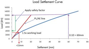
Given the good settlement performance of the pile, the same 24-inch (600mm) diameter pile is now shortened to 46 feet (14m) and numerically simulated to produce a load-settlement curve (Figure 6). The load is specifically chosen to load it beyond producing a settlement of 2.4 inches (60mm). Some codes (e.g., CP4 – Code of Practice for Foundations, Singapore) have recommended that the ultimate bearing capacity of piles be taken as 0.1D, where D is the pile diameter. In the U.S., a common way to define failure load is the load producing a settlement of (PL/AE + 0.15 + D/120) in inches, where D is the pile diameter. This is known as the Davisson method and can also be found in NAVFAC DM7-02 – Foundations and Earth Structures. Hypothetically, the working load can be found by reading off the ultimate load (2,700 kips or 12,000 kN) on the load-settlement curve at 0.1D and applying an appropriate safety factor to derive the working load of 900 kips (4,000 kN). However, at 1.5 times the working load of 1,350 kips (6,000 kN), the settlement exceeded 0.6 inch (15mm), which is not allowed by the same code. If 450 kips (2,000 kN) were to be taken as the working load, the settlement at 670 kips (3,000 kN), at 1.5 times, is less than 0.6 inch (15mm), which satisfies the settlement requirement. Note from Figure 5 that the PL/AE line provides a very crude under-estimation of the settlement at low loadings. It appears that a 46-foot (14m) pile is possible.
A quick calculation with assumed correlated shaft resistance and end-bearing values shows that a 46-foot (14m) pile is possible if a relatively high shaft resistance is used. Therefore, it is necessary to compare against actual shaft resistance and end-bearing obtained from an instrumented load test to verify that such values are indeed achievable. Similarly, the pile’s actual 1.5 times working load settlement should be checked.
Summary
Numerical simulations are often a valuable and powerful tool to gain insights into a problem and examine “what-if” scenarios that are impossible or impractical to perform in real-life situations. One example is the simulation of pile behavior under loads. It is possible to obtain reasonable shaft resistance and end-bearing values from a numerical model. Pile settlement can be readily calculated using numerical simulations, even with layered soils, which would be tedious to carry out by hand. With software, mathematical manipulations and number crunching are relegated to the back end. What is required is proper problem definition and the ability to capture the pertinent and peculiar features of a problem prominently and meaningfully in a model. A graphical interface provides immediate visual feedback on how the soil and pile behave. In addition, a qualitative examination of the displacements, load, stress, strain, and plastic point plots is often useful in deciphering whether a model responds or performs within expectations.
However, it is very easy to make mistakes when running a computer model, including arithmetic or other input errors. Moreover, numerical results generated are very much dependent on the input, such as boundary conditions, constitutive models, strength and deformation parameters, selection of interface thicknesses, etc. Deep scrutiny into the input is necessary before relying on or trusting the output or numerical value for any critical design decision. Therefore, it is often good practice to carry out benchmarking (against known or established results) and sensitivity studies (by varying key parameters within a range) to ensure numerical simulations do not produce results that defy logic and science. Despite convincing results from any numerical simulation, actual site measurements remain an instrumental part of pile design that should not be overlooked.■