If a man will begin with certainties, he shall end in doubts; but if he will be content to begin with doubts he will end in certainties.
– Francis Bacon
Practicing structural engineers must make decisions on safety, cost and utility even when “hard information” is not available. “Bayes’ Rule” is a mathematical tool for using experience and judgment to calculate the probabilities that could guide these decisions. The engineer assembles data such as test results, develops a hypothesis relating the data to underlying causes, and uses Bayes’ Rule to calculate the probability that the hypothesis is correct.
Bayes’ Rule is from a paper by Thomas Bayes published posthumously and later affirmed and augmented by Pierre-Simon Laplace. Recent applications of Bayes’ Rule, coupled with computer technology, have revolutionized statistical, scientific, and medical analyses (Iverson 1984, Mcgrayne 2011). This article shows how to use Bayes’ Rule with a spreadsheet program, such as Microsoft® Excel, to evaluate quality control sampling, test reports, reliability of bridge girders under random loading, office management decisions, and the Monty Hall Problem.
Using Bayes’ Rule requires an understanding of probability and statistics, and advanced applications can be challenging. Most textbooks on finite mathematics (Goldstein et al 2007) include an introduction to probability and Bayes’ Rule. There are also many Internet sources (Albert 2006). This article is at the introductory level. A derivation of Bayes’ Rule is included as an Appendix below.
Bayes’ Rule offers advantages over conventional statistics. The engineer may: 1) use subjective judgment or experience, based on the availability of test data; 2) update an analysis when new information becomes available; and 3) automatically calculate the probabilities of false positives (false alarms) and false negatives (missed defects or other items). False positives may increase cost, while false negatives may be disastrous. A high probability of either alerts the engineer that the test process may be wanting.
Probability and Statistics
“Probability” is a “fair bet” in a world of uncertainty. From statistics, P(A) = N(A) / N ≤ 1, where N is the total number of outcomes of an event, N(A) is the number of outcomes leading to A, and P(A) is the fraction (probability) of the total number of events in which A occurs. Given S as a subset of N, and (!) as the factorial symbol, the number of ways in which S items can be chosen from N possibilities is N!/[S! (N-S)!].
Low-strength concrete is a frequently encountered problem in construction. ACI 318 Section 5.6.2.1 (ACI 318- 08) requires at least one strength test for every 150 cubic yards (cy) of concrete placed each day, but not less than five strength tests for every class of concrete. If delivered in 5-cy capacity trucks, at least 30 trucks will be used to transport the concrete. If 10% of the concrete does not meet the ACI requirements, calculate the probability that the low-strength concrete truckloads would not be detected.
The number of ways of drawing five samples from 30 truckloads = 30!/(5! 25!) = 142,506. Assuming three truckloads of low-strength concrete (10% of 30), the number of ways of drawing five samples without low strength concrete = 27!/(5! 22!) = 80,730. P(A) = the probability of not detecting the low strength concrete = 80,730/142,506 = 0.567.
Bayes’ Rule Analyses
An “event” is the cause and its probability is called a “prior.” The engineer observes data T and uses Bayes’ Rule to calculate the probability of its relationship to a perceived cause. The probabilities of the observed effects, the data, are called “likelihoods” and may be based on experience, tests results, standard handbooks, or judgment. A Bayes’ Rule analysis follows these general steps:
- Propose a hypothesis P(E|T) relating priors and likelihoods.
- List available information about the priors, as probabilities.
- List the related likelihoods, as probabilities.
- Multiply the priors by the likelihoods, using Bayes’ Rule to calculate the “posterior probabilities.”
The posterior probabilities represent the probability that the hypothesis P(E|T) is true. The process is shown in the example problems. If the engineer has no relevant prior knowledge, a value of P(E) = 0.5 is recommended.
Example 1 – Quality Control Sampling
There are advanced applications of Bayes’ Rule in which the population data are the priors and the binomial distributions are the likelihoods. For this example, the HYPEGEOMDIST function in Microsoft Excel is more direct. In order, the inputs are the number of “successes” in the sample, the size of the sample, the number of successes in the population, and the size of the population. In this case, a “success” is actually not detecting low-strength concrete. HYPEGEOMDIST (0, 5, 3, 30) returns the correct value of 0.567.
Example 2 – Weld Inspection Report
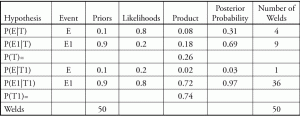
The engineer’s experience indicated that 10% of welds inspected by the specified test method would have defects. Laboratory reports from a project indicated that 20% of the 50 welds inspected to date had defects (Jordaan 2005). The engineer used Bayes’ Rule to analyze the situation. E was that a flaw was present in a weld and T was that the flaw would be detected by the specified test process. The hypotheses P(E|T) was that genuine weld flaws would be detected. Based on the engineer’s prior experience, P(E) = 0.1. The laboratory report indicated that P(T|E) = 0.8 and P(T1|E) = 0.2. From the Probability Sum Rule, P(E1) = 1- P(E) = 0.9, P(T|E1) = 0.2 and P(T1|E1) = 0.8. Calculating the posterior probabilities by Bayes’ Rule equations is cumbersome. If the factors are set up using a BAYES BOX (see Appendix), the calculation is more direct and convenient. The resulting posterior probabilities are identical to those calculated by using the Bayes’ Rule equations.
To interpret the results: The engineer expected 10% of the welds to have flaws; i.e., of the 50 welds inspected to date, five would have flaws (positive test results). The laboratory indicated that 20% of the welds (10 of 50) had flaws. The laboratory tests did not calculate the probabilities of false positives and false negatives. The Bayes’ Rule analysis calculated P(E|T) = 0.31, the probability that welds that tested positive would actually have defects. Of the 50 welds examined, four welds (0.31 x 0.26 x 50 = 4.03) would have “true” defects. P(E1|T) = 0.69, so about nine “defective” welds (0.69 x 0.26 x 50 = 8.97) would be false positives; that is, the test would have detected nine non-existing flaws. This was a statistical Type 1 error. Since P(E|T1) = 0.03, about one weld (0.03 x 0.74 x 50 = 1.11) had a flaw that the tests missed. This was a statistical Type 2 error. Finally, P(E1|T1) = 0.97, therefore the absence of flaws was correctly detected for about 36 of the welds (0.97 x 0.74 x 50 = 35.89).
The engineer would note that the combination of the probabilities of false positives and false negatives are indicators of the strictness of the testing system. Critical projects such as nuclear power plants need tight controls even though they are costly in time and budget. However, false negatives, flaws that were not detected in critical facilities, could be very hazardous.
If more test data becomes available, the posterior probabilities are used as priors in an updating analysis.
Example 3 – Bridge Girder Reliability (Monte Carlo Method)
The Monte Carlo method is used to evaluate the reliability, R, of a bridge girder subjected to random simulated loads. The random loading is applied iteratively until R converges. The number of iterations may range from hundreds to thousands. Microsoft Excel can generate over 30,000 iterations.
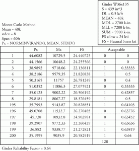
The bridge girder is a W36x135 spanning 60 feet, subject to a uniform dead load of 0.5 kips/foot and a concentrated live load at mid-span with a mean value of 40 kips. The engineer calculated the girder flexural stress using 200 simulated load tests assuming a normal distribution with a standard deviation equal to the mean divided by the square root of the number of samples, but not less than 1/5 of the mean (8 kips in this case). If this stress was less than or equal to the allowable value of 24 ksi, then the girder was considered acceptable. The reliability factor R of the girders was calculated as the ratio of the number of acceptable girders to the total number of girders (200). (Elishakoff 1999 pp. 440-41). (Spreadsheet details are in the Appendix.)
The results indicated a reliability factor R of 0.64, which does not significantly vary upon increasing the number of iterations. The engineer was confident about the adequacy of the girders and assumed P(E) = 0.95 (priors) accordingly, then used the R values as likelihoods in the Bayes Box analysis. P(E|T) is the probability that a girder meeting or exceeding R would be accepted.
The reliability of the bridge girders under random loading increased from 0.64 to 0.97 for girders meeting both E and T requirements (about 122 of 200 girders). However, the engineer noted from P(E|T1) = 0.91 that about 68 of the girders were “false negatives,” indicating that the engineer may be overconfident about the test process. As always, the engineer ultimately decides on the acceptability of R.
Example 4 – Office Management
4A. Bridge Collapse Preliminary Assessment
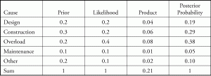
A bridge was being upgraded when it collapsed suddenly. A review of collapses of bridges of similar construction and vintage indicated the following probabilities of various causes: 0.2 by overload, 0.2 by design deficiencies, 0.3 by construction deficiencies, 0.1 by inadequate maintenance, and 0.2 by other causes. However, the engineer noted that at the time of collapse, one side of the bridge was open to normal traffic while the other was loaded with construction equipment. Accordingly, the engineer estimated a probability of 0.4 that the failure was due to an overload from the combination of construction loads and live loads. The other probabilities of failure were then assumed as 0.2 by design deficiencies, 0.2 by construction deficiencies, 0.1 by inadequate maintenance, and 0.1 by other causes. Calculate the probability P(E|T) for each cause of failure.
The probability of failure due to Overload increased from 0.2 to 0.38.
4B. Project Assignment
The supervising engineer considers both on-time performance and accuracy when assigning a project. Engineer A completed 70% of assigned projects on schedule, but there were major design changes required during construction on 40% of them. Engineer B completed 40% of projects on schedule, and only 10% of them required major design changes during construction. Assuming similar projects in scope and schedule duration, calculate the probability that each engineer would complete a project on schedule without major design changes.
Engineer A has a higher probability of completing a project on schedule and without major design changes.
4C. Monty Hall Problem
Suppose you are a contestant on a TV game show and are given the choice of three doors. Behind one of the doors is a prize, and behind the other two doors are goats. You pick a door. The host, who knows what is behind each door, then opens one of the other doors, showing a goat. You are allowed to change your door choice. Assuming you want the prize, do you change?
Using Bayes’ Rule, P(E) is the probability that the prize is behind your door = 1/3. P(E1) is the probability that the prize is behind one of the other two doors = 2/3. When the host opens a door that reveals a goat, the likelihood probability P(T|E) is the same that the prize is behind your door vs. the remaining door = 1/2.
Although it may seem counterintuitive, selecting the other remaining door, rather than the one you chose initially, actually improves your probability of winning to 0.67. This example illustrates the broad applicability of Bayes’ Rule and the importance of using both priors and likelihoods for a complete analysis.
Advanced Applications
Many advanced applications of Bayes’ Rule were supported by National Science Foundation funding and are available. They include structural responses to random excitations, decision analysis in building codes, uncertainty in model analysis, reliability of damaged structures, and random loading, from wind and seismic forces or terrorist attacks. Many additional articles and computer programs are on the Internet.
Conclusions
An engineer intuitively makes inferences based on available prior knowledge and related experimental data, while reserving the right to revise the inference based on new information. Bayes’s Rule is a vehicle for organizing this approach, a mathematical process for using experience and judgment to calculate the probabilities that could help guide engineering decisions. It tests both the “priors” and the “likelihoods”, while calculating the probabilities of an “E” and “T” hypothesis. In practice, the engineer would evaluate several sources of information, such as the qualifications of the testing laboratory, test records, etc., before making a critical decision.
The premise underlying Bayes’ Rule, as well as all education, is learning from experience and judgment. Bayes’ Rule reminds us that attempts to predict the future responsibly are possible only in terms of probability and that the highly improbable may occur. As always, the engineer is the one who ultimately decides.▪
References
ACI Committee 318, Building Code Requirements for Structural Concrete ACI 318-08 and Commentary, American Concrete Institute, Farmington Hills MI, 2008.
Albert, J. A Bayesian Primer, Key College Publishing, 2006.
Elishakoff, I., Probabilistic Theory of Structures, 2nd Ed., Dover Publications, Mineola NY, 1999, pp 440-41.
Goldstein, L.J., Schneider, D.I., and Siegel, M.J., Finite Mathematics and Its Applications, Pearson Prentice Hall, 2007, pp 273-457.
Iverson, G.R, Bayesian Statistical Inference, Sage Publications, Newbury Park, 1984.
Jordaan, I. Decisions Under Uncertainty, Cambridge University Press, 2005, pp 49-52.
Mcgrayne, S. The Theory That Would Not Die. Yale University Press, New Haven 2011.
Appendix
Bayes’ Rule
E = the event E occurs.
P(E) = the probability that event E occurs.
E1 = the event E does not occur.
P(E1) = the probability that event E does not occur.
E and E1 are “known” based on experience or estimated using judgment, and P(E) and P(E1) are called “priors.”
P(E) + P(E1) = 1.
T = a positive test result.
P(T) =the probability that T occurs.
T1 = a negative test result.
P(T1) = the probability that T1 occurs.
P(T) and P(T1) are based on actual observations and are called “likelihoods”.
P(T) + P(T1) = 1.
Note that E and T are independent events.
P(T|E) = conditional probability that T occurs given that E also occurs.
P(T|E1) = conditional probability that T occurs even though E does not occur (false positive).
P(T1|E) = conditional probability that T1 occurs even though E has occurred (false negative).
P(T1|E1) = conditional probability that T1 occurs given that E does not occur.
By the Probability Sum Rule, P(T|E) + P(T1|E) = 1 and P(T|E1) + P(T1|E1) = 1.
By probability rules, P(E|T) x P(T ) = P(T|E) x P(E).
Rearranging, P(E|T) = P(T|E) x P (E) / P(T) , which is Bayes’ Rule, given P(T) > 0.
P(T) is a normalizing factor = P(E) x P(T|E) + P(E1) x P(T|E1).
The usual form of Bayes’ Rule is: P(E|T) = P(T|E) x P(E) / [P(T|E) x P(E) + P(E1) x P (T|E1)].
Other forms of Bayes’ Rule are:
P(E1|T) = P(T|E1) x P(E1) / [(P(T|E1) x P(E1) + P(E) x P(T|E)].
P(E|T1) = P(T1|E) x P(E) / [(P(T1|E) x P(E) + P(E) x P(T1|E1)].
P(E1|T1) = P(T1|E1) x P(E) / [(P(T1|E1) x P(E) + P(E) x P(T1|E)].
By the Probability Sum Rule, P(E|T) + P(E1|T) = 1 and P(E|T1) + P(E1|T1) = 1.


