
A Practical Approach
Historically, equivalent static analysis procedures have been used to determine seismic design forces for conventional structures. In certain situations involving critical or highly complex structures, modal analysis procedures utilizing the elastic response spectrum concept have been employed. Both of these analysis procedures are computationally inexpensive yet they can be overly conservative. Recently, with the advent of performance-based seismic design concepts coupled with the significant advances in computing technology, the structural engineering community has shown a growing interest in seismic response history analysis. What has not been well documented is a clear procedure to find, select, and scale seismic time histories for use in a code-based design. This article outlines one such procedure that will enable a design engineer to access seismic time history databases, select the appropriate time histories for a given site and structure, scale these histories to ASCE 7 levels, and create a design based on ASCE 7 Chapter 16 procedures.
Selecting Ground Motion Histories
Perhaps the most important and challenging step in a seismic response history analysis is the proper selection of input ground motion histories to be used for subsequent dynamic analysis. It is highly recommended that both the structural and geotechnical engineer – and even a seismologist in some cases – participate in the selection process, as there are many multidisciplinary aspects that warrant consideration. Although the general, qualitative procedure for selecting appropriate input ground motion histories is essentially the same for any site, there are many quantitative details and nuances that can be specific to the governing regulatory documents and/or building codes as well as the specific site of interest. As such, this article will focus predominately on the general procedure.
Earthquake induced ground motion histories are non-periodic and highly nonlinear digitized curves that represent the kinematic response of a fixed point in the propagating medium or on the ground surface. The ground motion histories are influenced by things such as the characteristics of the seismic source, the fault rupture process, the geologic medium through which the seismic waves are propagating, and local site conditions. Fortunately, it is not necessary to predict every peak and trough of a ground motion history derived from a postulated earthquake event in order to successfully analyze and design a structure. Rather, it is necessary to identify key ground motion parameters that adequately reflect the characteristics of the ground motion: the amplitude, duration, and frequency content of the motion. The peak horizontal acceleration is historically the most popular amplitude parameter used to describe a ground motion – largely due to its inherent relationship with inertial forces. Ground motion duration is another important parameter that tends to get less attention than others, and can have a significant influence on structural damage. The most common duration parameter is arguably the bracketed duration, which is defined as the time between the first and last exceedance of a threshold kinematic response quantity. The frequency content of a particular ground motion provides information about relative energy demand as a function of individual signal frequencies, and it can be most clearly depicted in a Fourier amplitude spectrum. Another measure of frequency content that is often employed in the commercial nuclear energy industry is the power spectrum or power spectral density function (e.g., ASCE 4-98). By far, the most popular frequency domain spectrum utilized in earthquake engineering practice is the elastic response spectrum (ERS). An ERS describes the maximum elastic response of a single-degree-of-freedom (SDOF) system to a given ground motion history as a function of the SDOF system’s natural frequency and critical damping ratio. The ERS contains a spectral response quantity on the ordinate axis (spectral acceleration, velocity, or displacement) and SDOF system natural frequency or period on the abscissa axis. Although the ground motion characteristics are filtered by the response of the SDOF system, it is important to point out that the amplitude, frequency content, and (to a lesser extent) duration of the input ground motion are all reflected in the spectral response values.
The first step in the general procedure for selecting ground motion histories is to conduct a seismic hazard analysis to determine the control points of the design basis ERS (e.g., ASCE 7-10 Fig. 11.4-1). For typical structures located on geologically favorable sites, the seismic hazard analysis and determination of the design basis ERS control points can be done per the ASCE 7-10 Section 11.4 provisions along with the seismic ground motion long-period transition and risk coefficient maps of ASCE 7-10 Chapter 22. This process can be expedited by utilizing the United States Geological Survey’s U.S. Seismic Maps Web Application. For critical facilities, such as disaster response facilities and mission-critical military structures or structures located on soils vulnerable to potential failure or collapse under seismic loading (e.g., liquefiable soils), a rigorous site-specific probabilistic seismic hazard analysis and site response analysis may be required.
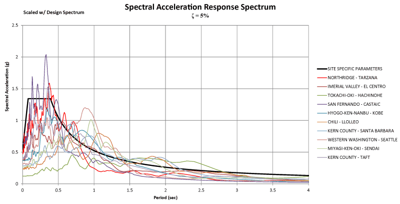
Figure 1: Example elastic response spectrum.
Once the design basis ERS is established, the next step is to obtain or generate ground motion histories that possess sufficiently similar ground motion characteristics as those exhibited by the design basis ERS. The most common method to measure compatibility between the ground motion histories and the design basis ERS is to overlay the ground motion history ERS with the design basis ERS (Figure 1). Most building codes and regulatory documents acknowledge the uncertainties associated with “seismically similar” ground motion histories by requiring more than one set of ground motion histories to be considered during analysis. Ideally, actual recorded ground motion histories from recording stations near the site of interest exist. A detailed list of websites containing national and international strong motion data can be found on the MCEER website. When this is the case, these baseline histories should first be compared with the design basis ERS. If adequate compatibility is not achieved, then the ground motion histories can be carefully scaled to fit the tolerances of the design basis ERS. If no suitable ground motion data exist, then the generation of synthetic ground motion histories is usually permitted. A synthetic ground motion history can be developed in one of three ways: time domain generation, frequency domain generation, or by Green’s Function techniques. For a more thorough treatment of ground motion selection and scaling, it is recommended that the NIST GCR 11-917-15 Selecting and Scaling Earthquake Ground Motions for Performing Response-History Analyses be consulted.
Developing an Elastic Response Spectrum
Once the ground motion histories have been selected or synthetically generated, the ground motion ERS’s are computed and compared to the design basis ERS to ensure their compatibility. As discussed previously, an ERS describes the maximum elastic response of an SDOF system to a given ground motion history. The equation of motion can be solved using numerical time integration methods where the equation is integrated using a step-by-step procedure. The equation of motion to be solved numerically can be cast as shown in Equation 1,
[pmath]{d^2}/{dt^2}[/pmath]u(t) + 2ωξ [pmath]d/dt[/pmath]u(t) + ω2u(t) = –ag(t)
(Equation 1)
where, u(t) is the relative displacement of the SDOF system with respect to the ground displacement, ag(t) is the ground acceleration, ω is the SDOF natural frequency (rad/sec), and ξ is the SDOF critical damping ratio. The relative displacement and ground acceleration are both functions of time corresponding to the history’s recorded time steps. There exists a large body of knowledge regarding solution methods for various types of differential equations. For purposes of this article, only two common methods useful in dynamic response analysis will be briefly discussed; the Central Difference Method (CDM) and the Newmark Method. The CDM is probably the most common explicit numerical integration technique employed to solve dynamic response problems, but it is only conditionally stable – meaning that if the selected time step is not short enough then the solution will diverge rendering erroneous results. The Newmark Method is an implicit numerical integration technique, and it is unconditionally stable when the average acceleration approach (as opposed to the linear acceleration approach) is taken. Both methods are presented in detail in almost any structural dynamics text, but they are only introduced here to assist in understanding the creation of an ERS. An example using Newmark’s Average Acceleration Method will be used to demonstrate the required steps to develop an ERS (Figure 2). The example provides the readers with definitions of terms, useful relationships and initial calculations to aid in the development of an ERS for a specific acceleration time history.
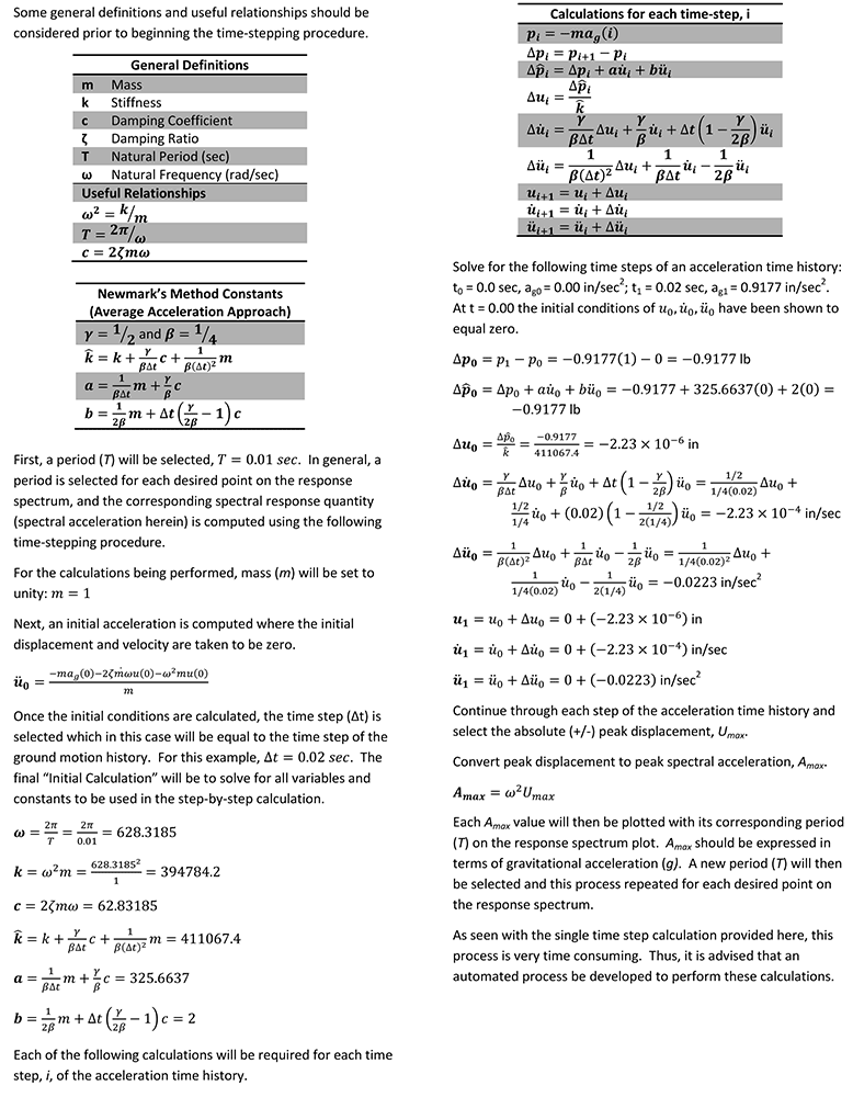
Figure 2: Newmark’s average acceleration method example.
ASCE 7-10 Code Requirements
Once an ERS has been created from a selected ground motion history, the engineer can begin to compare the record to a code level event. Different histories will create vastly different ERS’s due to the natural variation of frequency and acceleration content within the records themselves. This will typically result in a highly variable response spectrum (unlike the smoothed spectrum found in Section 11.4.5 of ASCE 7-10). The general shape of the response spectrum for most records will share a shape similar to the design spectrum (for certain records, however, this is not the case, and significant deviations from the design spectrum are possible).
Given the rarity of Maximum Considered Earthquake (MCE) level events, it is common to scale specific acceleration records to match an MCE level event for a given site. Many different techniques for scaling records exist, each with their own benefits and drawbacks. The available techniques largely fall into two broad categories; techniques that modify the frequency content of a record and those that do not. Of the two categories, techniques which allow modification of the frequency content are much more demanding and hence beyond the scope of this article. To this end, the authors will focus on the application of a simple uniform amplitude scale factor which generally produces satisfactory results.
Aligning the ground motion history ERS within a code-specified tolerance of the design basis ERS control points ensures similarity in ground motion amplitude, frequency content, and duration. Per Section 16.1.3.2 of ASCE 7-10, “Each pair of motions shall be scaled such that in the period range from 0.2T to 1.5T, the average of the SRSS spectra from all horizontal component pairs does not fall below the corresponding ordinate of the response spectrum used in the design.” As described earlier in this article, an ERS must first be created for each record using 5 percent critical damping. The response spectrum ordinates of the two component pairs of each record must then be combined using the square root of the sum of the squares (SRSS) method. The ordinates of these new SRSS spectra for each set of component pairs are then averaged together to create a single averaged ground motion ERS. This averaged ground motion ERS is then compared to the design basis ERS of Section 11.4.5 of ASCE 7-10. Scale factors are then selected and applied to the ordinates of each pair of records to ensure that the ordinates of the averaged ground motion ERS do not fall below the design basis ERS within the period range of 0.2T to 1.5T. It should also be noted that when dealing with two orthogonal horizontal component motions for use in a coupled 3-dimensional dynamic analysis, it is often required that one component motion be statistically independent from the other. For example, when selecting/developing ground motion histories for a commercial nuclear energy facility, ASCE 43-05 requires that the directional correlation coefficients between pairs of records be less than or equal to 0.30.
Although ASCE 7-10 provides no specific guidance on the selection of individual scale factors, and an engineer could conceivably meet the provisions by applying a very large scale factor to a few records and a small factor to the remaining records, this is not in agreement with the general intent of the provisions. The authors recommend selecting an initial scale factor that satisfies the following relationship:
∫[pmath]{1.5T}under{0.2T}[/pmath][f(x)–n*g(x)] dx≅ 0
(Equation 2)
where, f(x) is the design basis ERS, g(x) is the averaged ground motion ERS, and n is the scale factor. After the selection of an initial scale factor, small adjustments can be made to meet the provisions of Section 16.1.3.2 of ASCE 7-10. It is worth noting that the use of large scale factors (the authors suggest n≤5 as a rule of thumb) should be avoided if possible. The validity of a record that requires a very large scale factor is somewhat reduced, especially when the source mechanism is not consistent with the MCE level event.
Once a record has been selected and scaled to the appropriate level, it can be used to perform a code level analysis and/or design. Chapter 16 of ASCE 7-10 recognizes two primary methods of response history analysis: linear and nonlinear. A linear analysis requires additional scale factors to be applied to the analysis results whereas the results of a nonlinear analysis do not require additional scaling. Per Section 16.1.4 of ASCE 7-10 for a linear analysis, “force response parameters shall be multiplied by Ie/R” and “Drift quantities shall be multiplied by Cd/R.” These factors approximate the effects of material nonlinearity that are not captured directly by the linear analysis. Additionally for a linear analysis, “where the maximum scaled base shear predicted by the analysis, Vi, is less than 85 percent of the value of V determined using the minimum value of Cs set forth in Eq. 12.8-5 or when located where S1 is equal to or greater than 0.6g, the minimum value of Cs set forth in Eq. 12.8-6, the scaled member forces, QEi, shall be additionally multiplied by [pmath]V/{V_i}[/pmath].” This factor is meant to safeguard from inappropriately flexible building models (and other analysis errors) leading to artificially low base shears.
For both linear and nonlinear analysis, if at least seven ground motions are analyzed then it is acceptable to use average response values for design. If fewer than seven ground motions are analyzed – ASCE 7-10 requires a minimum of three ground motions – then the maximum response values must be used for design. When performing a three-dimensional analysis, these ground motions should consist of horizontal matched pairs selected based on the aforementioned statistical requirements. For a two-dimensional analysis, these ground motions shall consist of a single horizontal ground motion history.
The use of the seismic overstrength factor (Ω0) is also modified when performing a response history analysis. Chapter 16 of ASCE 7-10 contains two different provisions regarding the use of the seismic overstrength factor depending on whether a linear or nonlinear analysis is performed. Per Section 16.1.4 of ASCE 7-10, the seismic load effects including the over strength factor for a linear analysis need not be taken larger than the maximum unscaled value obtained from the linear analysis. Per section 16.2.4.1 of ASCE 7-10 for a nonlinear analysis, “the maximum value of QEi obtained from the suite of analyses shall be taken in place of the quantity Ω0QE.” This can have a significant effect on the design of a structure located in a region of high seismic risk.
Conclusion
The provided commentary, external references, and examples have been assembled in an attempt to raise awareness in those engineers who stand to benefit from the use of seismic response history analysis. It is the hope of the authors that this article will provide the reader with an increased awareness of seismic response history analysis and serve to diminish the perceived barriers to its use.▪